1   Introduction¶

We aim to create a point spread function (PSF) model for Hyper Suprime-Cam (HSC) that separates the contribution of optics from the contributions of sensors and the atmosphere. “Optics” in this context includes all of: aberrations built into the HSC design, deviations from that design in the realized surfaces, misalignments of surfaces, and non-flatness of and discontinuities between the detectors populating the HSC focal surface. Modeling the sensor discontinuities is of particular interest, as these introduce discontinuities into the final delivered PSF. These discontinuities restrict current PSF interpolation algorithms to operating on single CCDs at a time. By modeling the discontinuities, we hope to enable interpolation of the non-optical PSF components across the entire focal plane.

We assume that the optics design, deviations in the realized surfaces, and sensor discontinuities can all be characterized in a single reference wavefront. Misalignments will in general vary from exposure to exposure, as the telescope and camera experience different gravitational loads, temperatures, and potentially hysteresis. The added effects due to misalignments on the wavefront should be slowly varying in degree of misalignment, and pupil and focal coordinates. We believe we can model these effects with a small number of parameters for every individual exposure.

In this technote, our goal is to demonstrate that we can measure the HSC wavefront from out-of-focus “donut” images of stars, and that we can use this wavefront to predict the optical component of in-focus PSFs. We make this validation using both simulations and observations on donut and in-focus images.

2   Forward Model¶

We assume a monochromatic Fourier optics description of the optical part of the PSF:

In the above, \(I(\theta, x)\) indicates the PSF, \(\theta\) indicates a position on the sky where the PSF is evaluated, and \(x\) is the variable used to describe the surface brightness variation of the PSF itself. I.e., for a single point source, there is exactly one \(\theta\), but a range of relevant \(x\).

\(P(\theta, u)\) is the pupil obscuration function. This is a binary-valued function indicating which paths are obscured (value = 0) or unobscured (value = 1) going from the pupil plane to the focal plane. In principle, it is the exit pupil which matters here, which for HSC is a virtual surface located behind the camera. In practice, however, we can think of the coordinates \(u\) as residing on the entrance pupil, which is roughly equivalent to the primary mirror. Which paths are obscured/unobscured depend on their entrance angles \(\theta\).

The wavefront \(W(\theta, u)\) indicates the lead or lag of the realized wavefront from an ideal spherical wavefront converging to a point on the focal surface (the particular point depends on \(\theta\)). The second equation indicates how we model the wavefront: as a series expansion of Zernike polynomials \(Z_j(u)\) with coefficients \(a_j(\theta)\). We start at \(Z_4\) because this is the first Zernike term that actually affects the profile of the PSF (\(Z_1\) is a phase term, the effect of which completely disappears after the \(|\cdot|^2\) operation, and the \(Z_2, Z_3\) terms are perfectly degenerate with coordinate origin shifts). For the moment, we will leave the functional form for the field angle \(\theta\) dependence of the Zernike coefficients unspecified, though this will be important when we develop the wavefront model separating static effects and dynamic effects eluded to above.

The \(\mathfrak{F}\) indicates a Fourier transform; in this case an integral over \(u\) producing a function of \(x\). Finally, \(\lambda\) is the wavelength of light in the model. For the moment, we assume that the optics PSF can be adequately modeled monochromatically using the effective wavelength of whichever filter is being analyzed.

In the above, \(\theta\), \(x\), and \(u\) are all 2-dimensional vectors.

The normalization of the optical PSF is assumed to be such that the integral over all of space (i.e., over \(x\)) is unity. This convention for PSFs is generic, extending to the final PSF which also includes contributions from the atmosphere and sensors. Flux information in an image will be carried by the surface brightness profile of the object being convolved by the PSF, which may be a (non-unit) delta function in the case of a star, or a more complicated profile in the case of an extended object.

2.1   Donut PSFs¶

The final delivered PSF also includes contributions from sensors (primarily in the form of charge diffusion), and the atmosphere. The atmospheric component nominally follows from the same Fourier optics formalism as the optics component, with the main differences being that the atmospheric wavefront aberrations are typically much larger than optical aberrations and they evolve on scales of milliseconds instead of being roughly constant during an exposure. An important consequence of this, combined with the nonlinearity of the equation for \(I(x)\), is that the time averaged wavefront is not simply related to the time averaged PSF.

In order to develop our wavefront-based optics PSF model, we need a way to measure the wavefront. Measuring the wavefront ab initio from in-focus data is nearly impossible due to the confounding atmospheric PSF (and limited resolution offered by the HSC pixel size). However, by defocusing the camera, we can amplify the effects of the optics wavefront while keeping the effects of the atmospheric PSF roughly constant. The caveat to this approach is that optical aberrations change when defocusing the camera. Fortunately, this change is linear, so an effective strategy is to measure both the intra-focal and extra-focal wavefront and average them together to get the in-focus wavefront prediction.

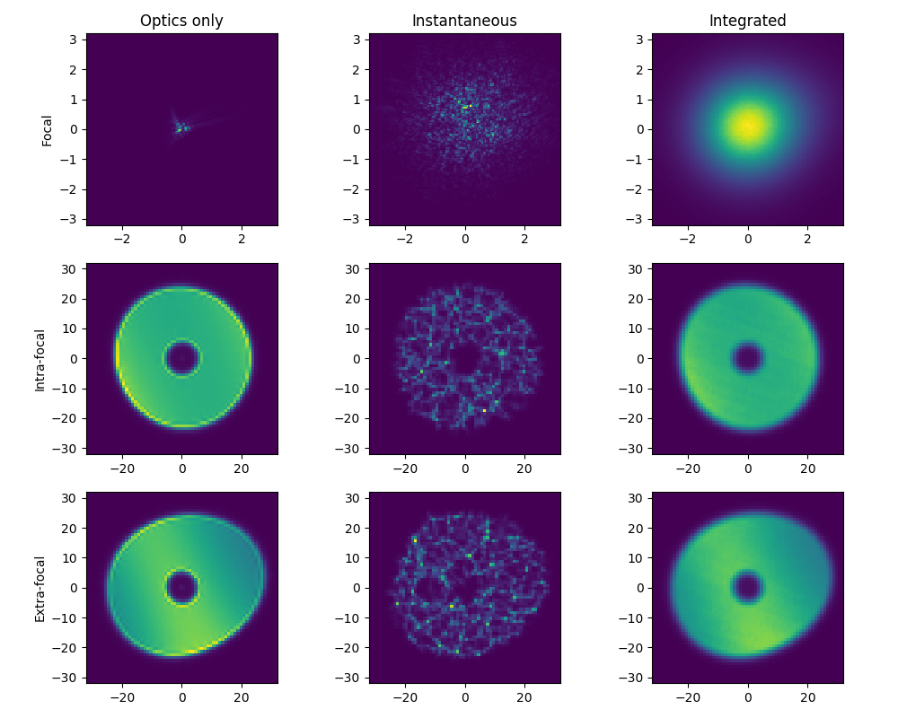
Figure 1 Illustration of how donut images enable optical wavefront reconstruction. Note the difference in scale between the rows. The first column shows simulated images including only optics effects. The non-circularity of the images (both in and out of focus) is related to non-circularity in the simulated wavefront aberrations. The second column shows the same simulation, but including atmospheric effects (but with an exposure time of 0 seconds). The change to the in-focus PSF is dramatic compared to the change in the donuts. The right column integrates the atmospheric effects over 15 seconds. While it would be very difficult to infer anything about the optics from the in-focus integrated image, the integrated donuts still retain most of the optics information. Simulation done in GalSim, the source code can be found in this technote’s repository.

3   Model validation in Zemax¶

To validate the wavefront-based PSF modeling, we used the commercial raytracing package Zemax and the S402C description of HSC and the Subaru telescope to simulate sets of intra-focal, extra-focal, and in-focus images. We used the Zemax HuygensPSF tool to simulate in-focus optical PSF images at a resolution of 0.25 \(\mu m\), which roughly corresponds to 0.0028 arcseconds at the mean HSC pixel-scale of 0.168 arcseconds per 15 \(\mu m\) pixel. To simulate donut images, we first displaced (in Zemax) the camera from the primary mirror by \(\pm 0.9 mm\) along the optic axis. We again used the HuygensPSF tool to generate an image, this time at the native pixel scale resolution of 15 \(\mu m\). To make these images more realistic, we used GalSim to convolve them by a Kolmogorov profile and add a small amount of uncorrelated stationary Gaussian noise (this extra convolution and noise addition also seems to help our fitter converge). We also used Zemax to determine the pupil obscuration function exactly.

After finding the wavefront coefficients by fitting the intra-focal and extra-focal donuts, we averaged them together to produce an inferred wavefront for the in-focus optical PSF. We then compared the inferred in-focus wavefront and PSF to the simulation truth obtained from Zemax.

We validated the forward model approach using 2 configurations of the simulated camera/telescope: one in which the optics are perfectly aligned, and one in which the camera is slightly shifted and tilted with respect to the primary mirror optic axis. We investigated 4 points in the field of view spanning the complete range in incoming field angle of 0 to 0.75 degrees.

The following multi-panel figures show the results for one of these images sets. In the particular set shown, the camera has been misaligned and the field angle is near maximal at 0.75 degrees.

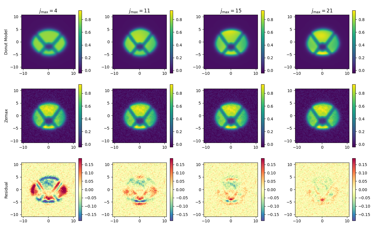
Figure 2 Intra-focal donuts fit validation. The top row shows forward model fits to the Zemax-simulated images using progressively more Zernike polynomials in the wavefront description. The middle row shows the particular Zemax donut being fit (each column is identical in this row). The bottom row shows the residuals. The analogous figure for extra-focal donuts is qualitatively similar, but omitted here for concision.

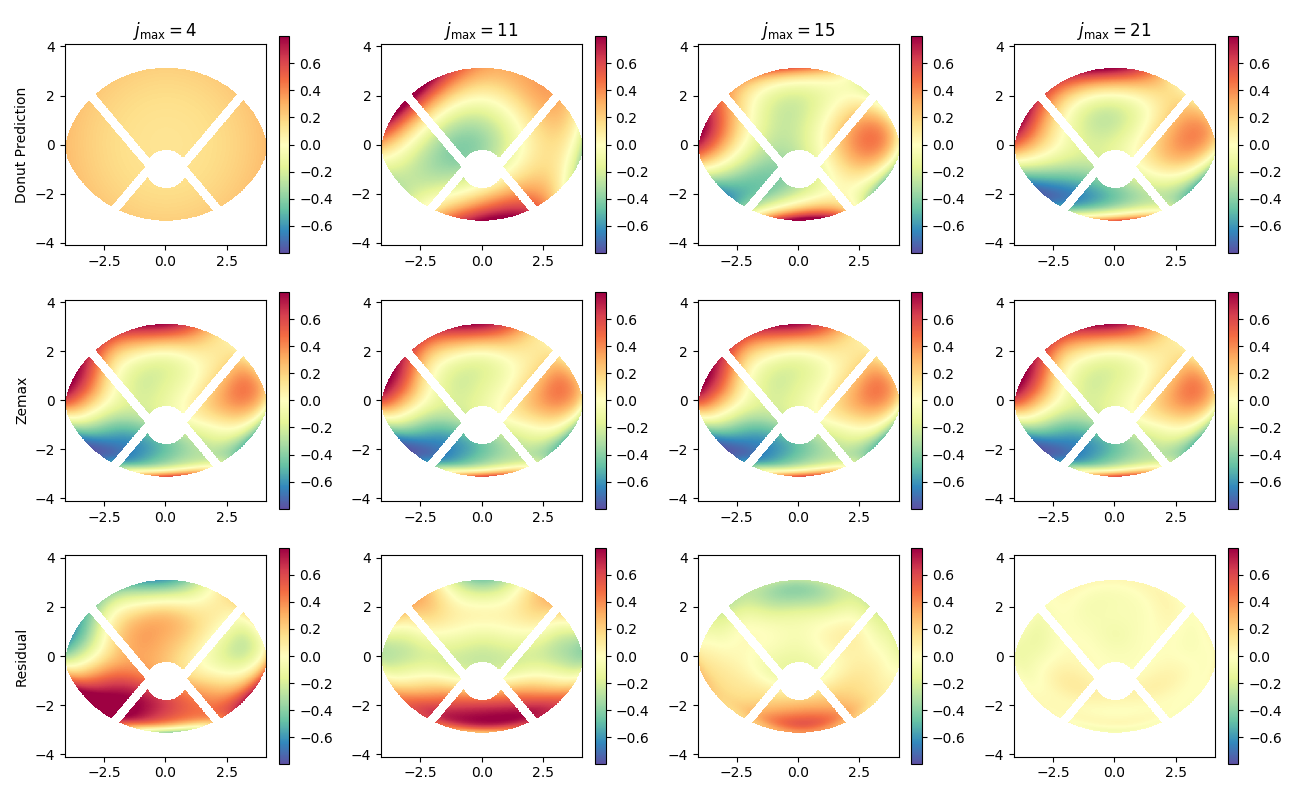
Figure 3 Wavefront inference validation. The top row shows the wavefront inferred from the donut image pairs using progressively more Zernike polynomials in the wavefront description. The middle row shows the true wavefront from Zemax. The bottom row shows the residuals.

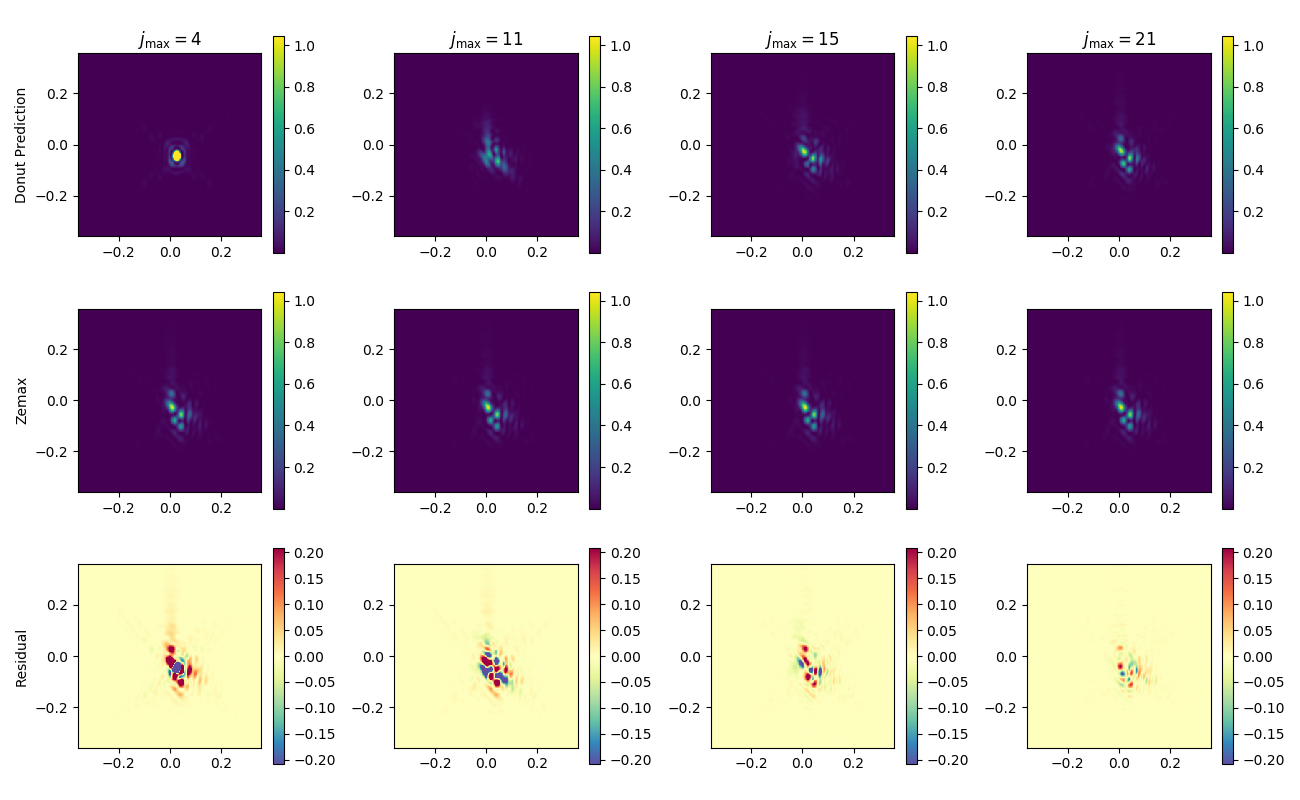
Figure 4 Optical PSF inference validation. The top row shows the optical PSF inferred from the donut image pairs using progressively more Zernike polynomials in the wavefront description. The middle row shows the true optical PSF from Zemax. The bottom row shows the residuals.

One important point here is that at no point did we do anything special to account for distortion in the optics. That is, the simulated images are created in physical units of mm (by Zemax), and in general have a nonlinear relationship with sky-coordinates or even a tangent plane projection thereof. Investigating the potential impact of distortion is on our list of open questions.

4   Model application to real data¶

To test the optical PSF model on real data, we rely on a set of HSC engineering images: visits 69008 through 69072. These images were taken in sets of three (which we will refer to as a “triplet”), alternating through an in-focus exposure, an extra-focal exposure (with camera displaced by +0.9 mm), and an intra-focal exposure (with camera displaced by -0.9 mm). Each exposure in a triplet was taken at the same location on the sky, which allows us to directly compare intra- and extra-focal donut images with in-focus PSFs for a fixed set of focal-plane locations, without needing to worry about interpolating across the focal plane. The telescope elevation and rotation angle were varied from one triplet to the next. All triplet images in this range were taken through the I2 filter.

4.1   Estimating the pupil obscuration function¶

Recall that we assume the pupil obscuration function \(P(\theta, u)\) is known a priori during a given wavefront fit. This function varies considerably across the HSC field-of-view due to the significant vignetting of the camera, and also has significant contributions from the telescope spiders and camera shadow.

4.1.1   Pinhole images¶

To estimate the pupil obscuration and its variation, we use a set of HSC images taken through a pinhole filter and illuminated by a flat screen. Each pinhole forms an image of the pupil on the focal plane. We choose to describe this image using a combination of three circles and four rectangles. The first circle is used to indicate the boundary of the primary mirror (shown in blue below). The second circle indicates the shadow formed by HSC itself (shown in green below). The third circle shows where rays are clipped by the first HSC lens (shown in red below). Using ds9, we match the edges of these circles to the edges formed by the pinhole images and record the positions of each circle center.

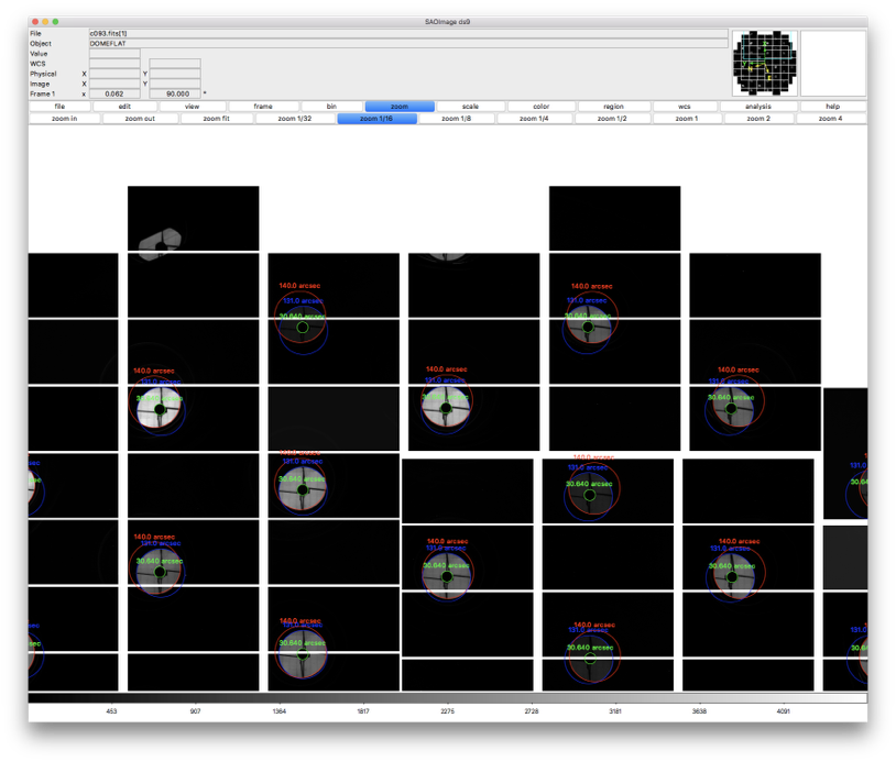
Figure 5 Screenshot showing images through pinhole filter and circles used to characterize the pupil.

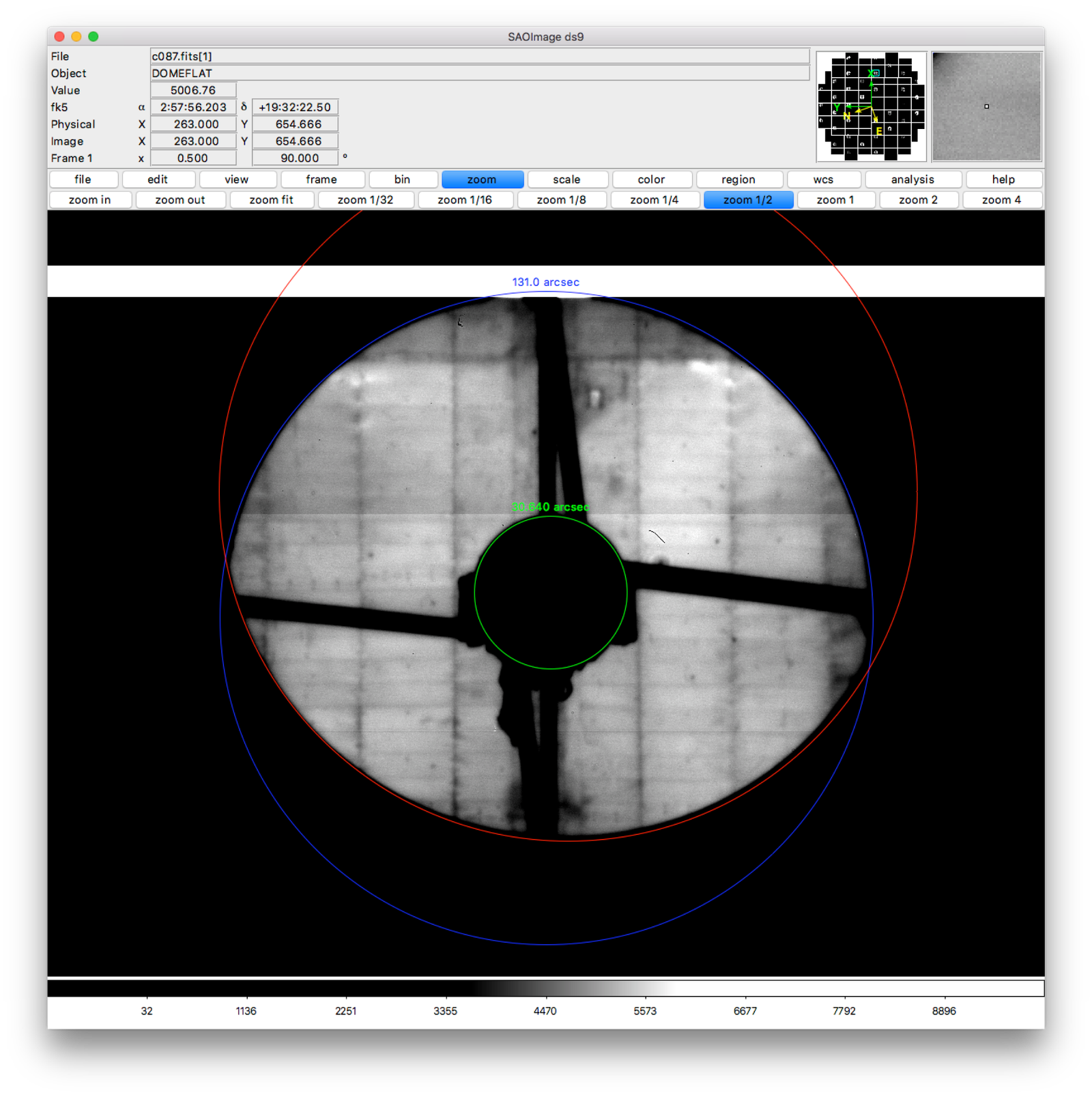
Figure 6 Zoom-in on one pinhole image and circles used to model pupil.

We next investigate how the circles centers relate to one another as a function of focal plane position. The plots below indicate that this variation is quite close to linear in the field radius.

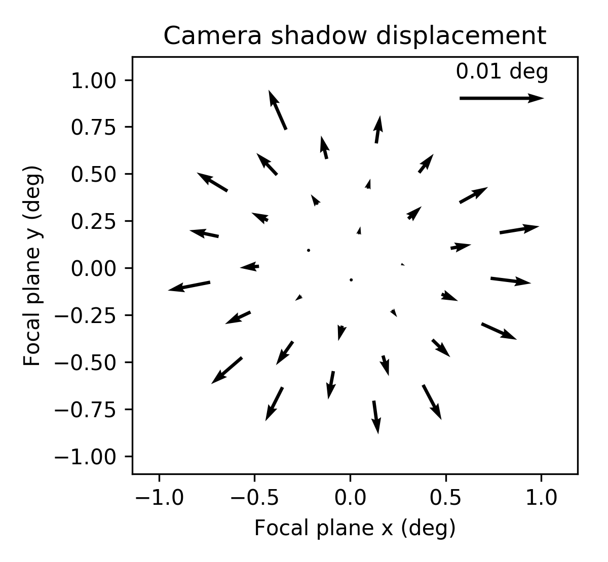
Figure 7 Camera shadow displacement with respect to primary mirror across the focal plane.

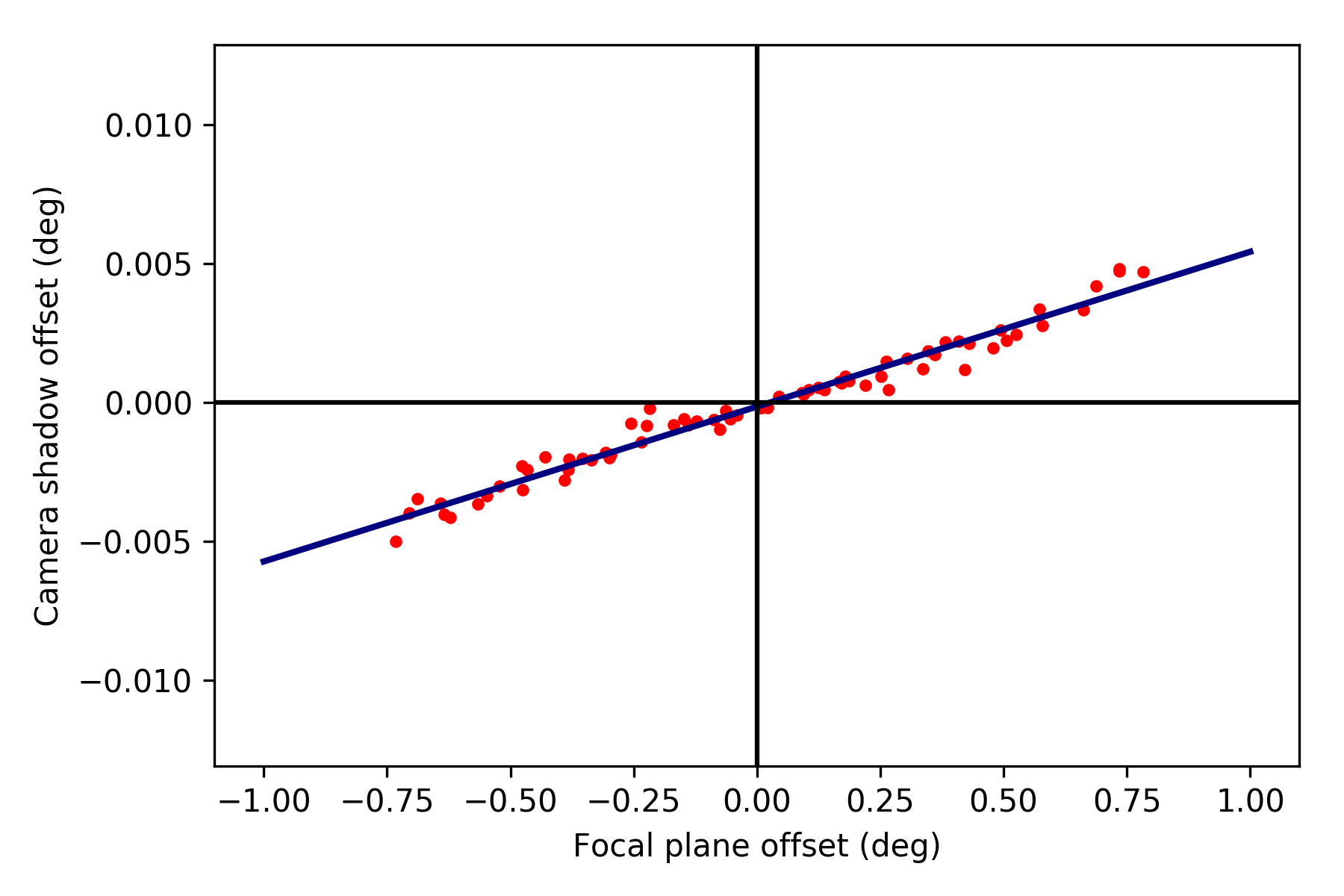
Figure 8 Camera shadow displacement radial fit.

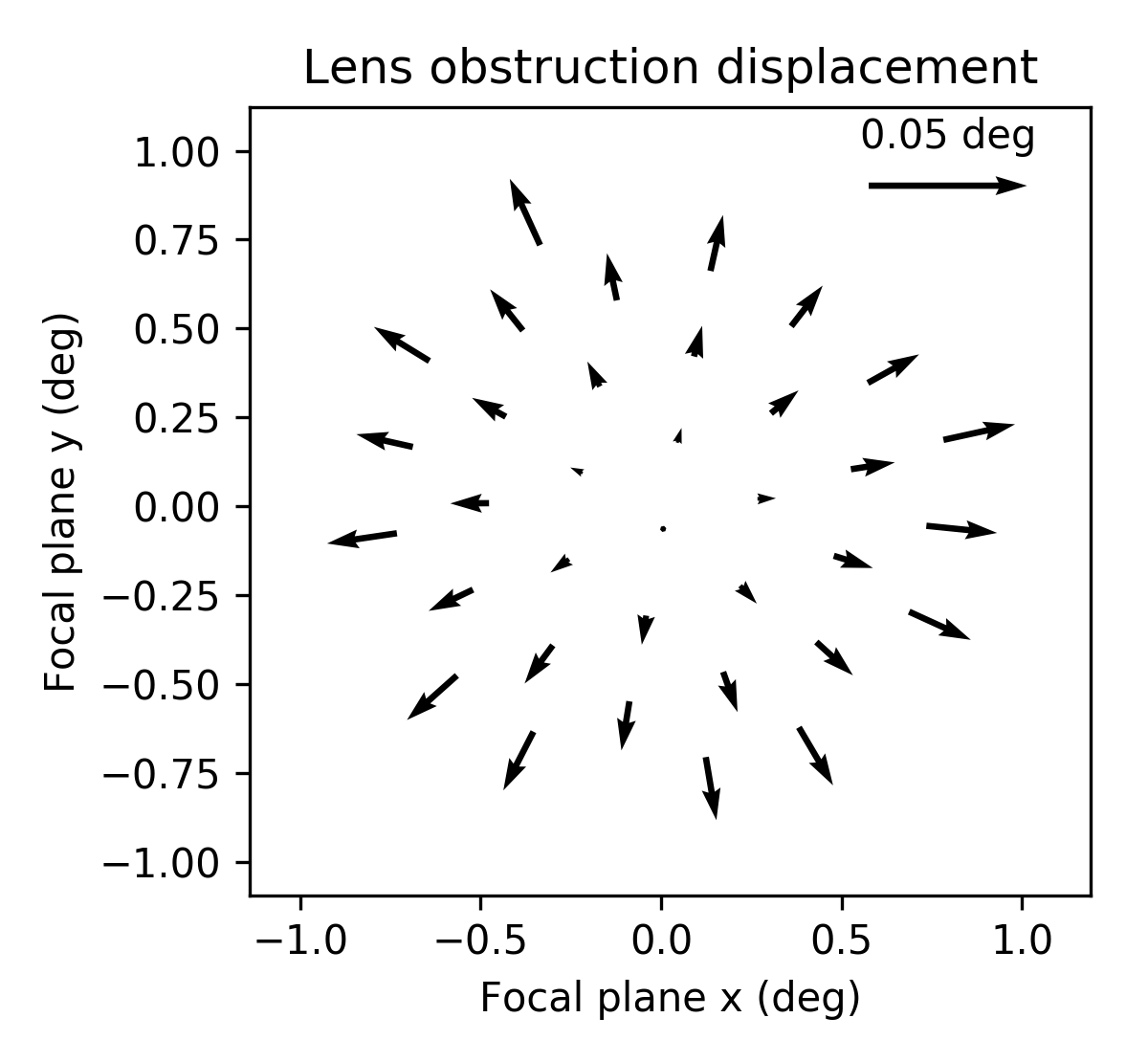
Figure 9 HSC lens clipping displacement with respect to primary mirror across the focal plane.

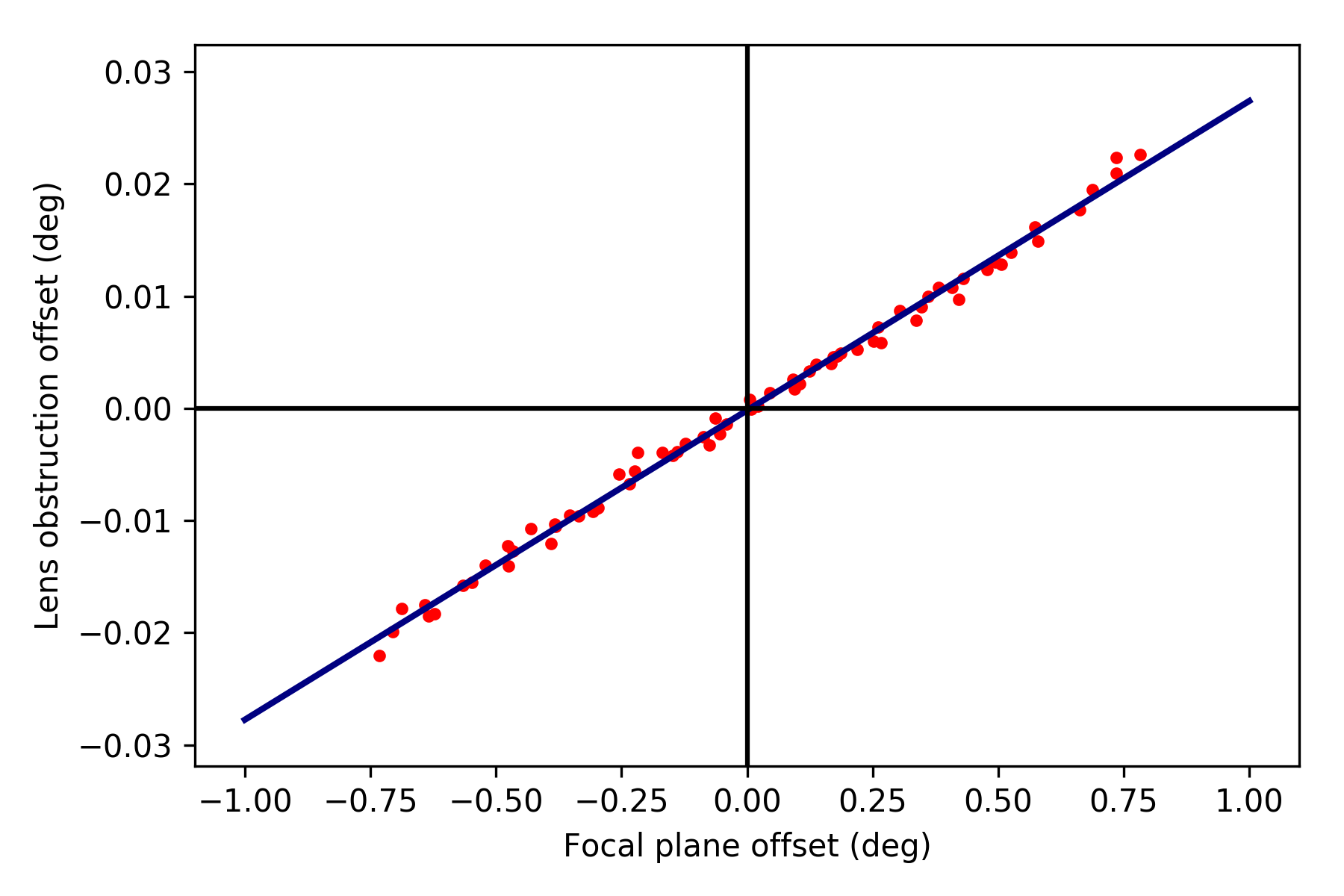
Figure 10 HSC lens clipping displacement radial fit.

4.1.2   Pinhole != pupil¶

While the pinhole images are a valuable source of data from the real HSC instrument, we note that the images formed this way are not strictly the same as the pupil. Each individual pinhole image is formed by light encountering the optics (specifically, the primary mirror) from a variety of angles, and then passing through the filter plane within a narrow transverse aperture (i.e., within the pinhole). By contrast, true pupil rays for a given field angle are initially parallel, and are unconstrained in the filter plane (although in practice, because the filter plane is near the focal plane, only a relatively small region of the filter will intersect the incoming beam for a given field angle). Using the raytracing software batoid, we have confirmed that this distinction does produce different pupil obscuration functions, though we have not, as yet, propagated these differences to see their potential impact on wavefront or PSF inference.

It should be possible to empirically measure the true pupil by using images of stars taken very far from focus (much farther from focus than the donut images analyzed below). As the defocus is increased, interference effects become insignificant compared to geometric effects, allowing the pupil to be cleanly observed.

4.2   Individual donut fitting¶

For measuring wavefronts, it’s important to select reasonably bright isolated objects that originate from point sources and not extended sources. To this end, we use three criteria to select donuts for further analysis:

1. High signal-to-noise ratio.
2. The donut “hole” is significant. This feature would be washed out for extended sources.
3. The object is not too large, which may indicate blending of neighboring sources.

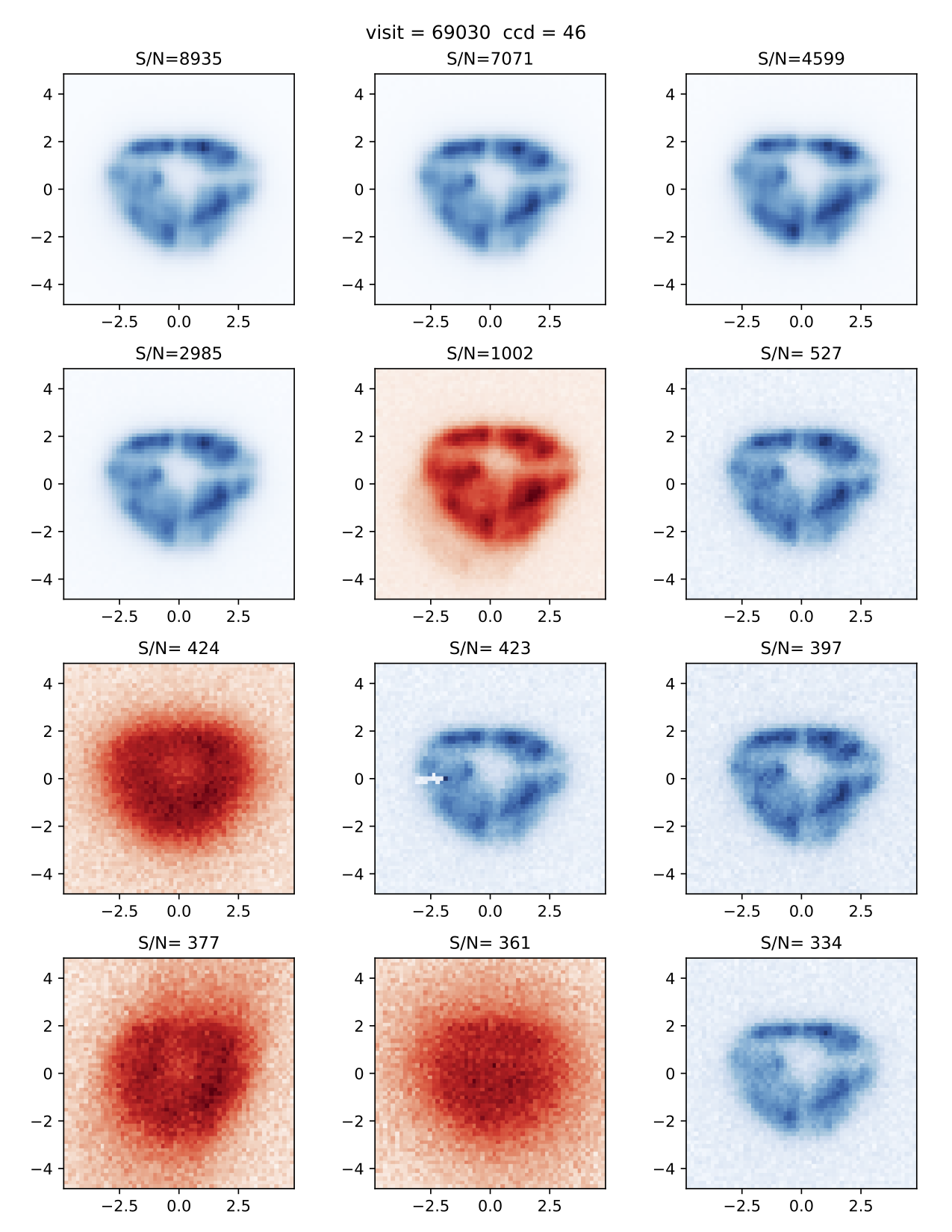
Figure 11 Example of donut selection. Green donuts are selected for fitting; red donuts are rejected. These particular donuts are from HSC CCD 46, which is located towards the edge of the HSC field of view. As such, there is significant vignetting visible. Notice the rejected donut in the second row, which has a visible blend. The other three rejected donuts clearly originate from extended sources. Also notice the unflagged artifact in the selected donut in the middle column of the third row. The fit to this donut may be unreliable.

We fit each selected donut independently using the model specified above. To improve the convergence of the model, we fit iteratively, increasing the value of \(j_\mathrm{max}\) in each iteration (from 4 to 11 to 15 to 21), and using the results of the previous iteration to initialize the parameter values for each subsequent iteration. Sample results for \(j_\mathrm{max} = 21\) are shown in the figure below.

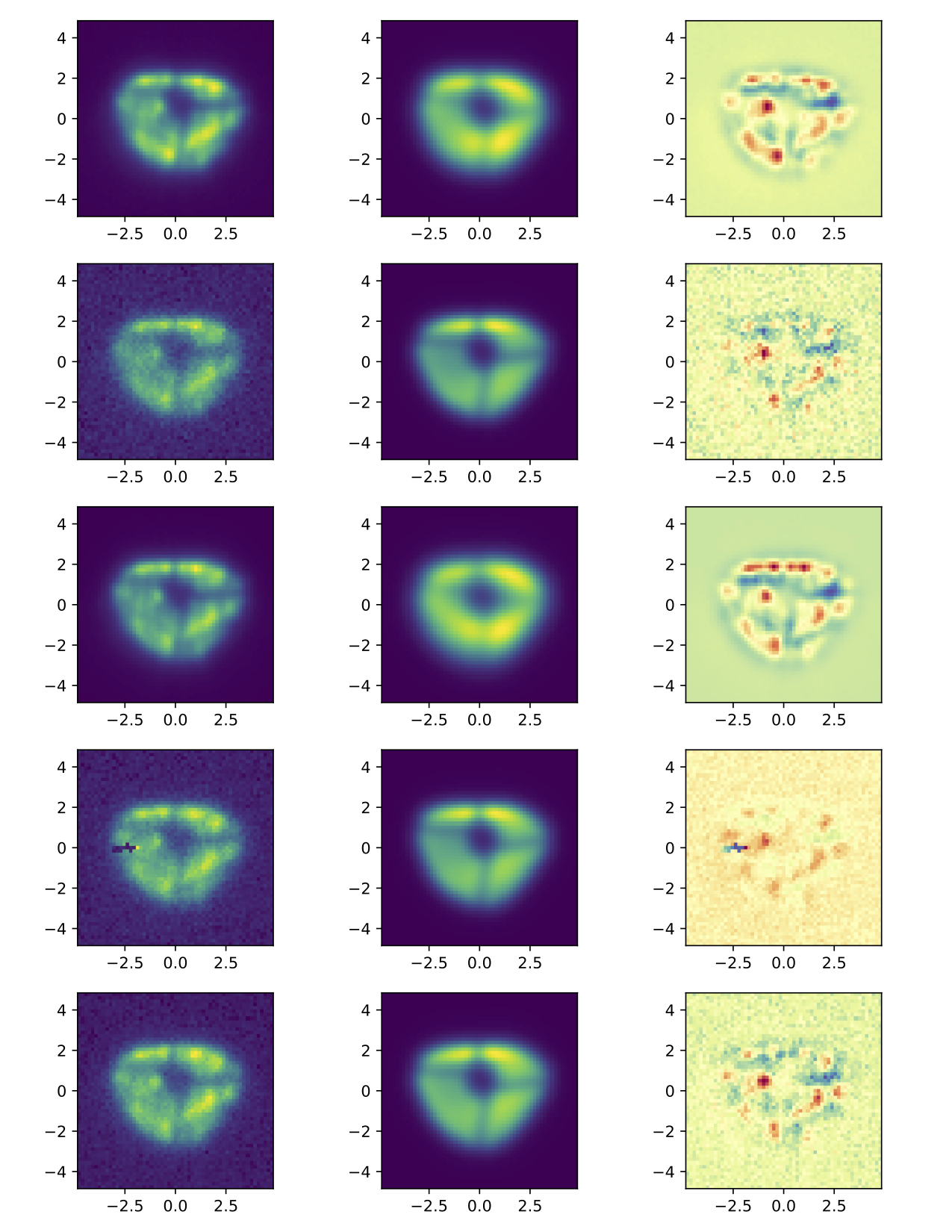
Figure 12 Example donut fits. The left column shows the data, the middle column shows the best fitting model, and the last column shows the residual.

While the fits are plausible, there is clearly structure in the data not being captured by the model. It may be possible to improve the fits by increasing \(j_\mathrm{max}\), at the expense of increased computational time to perform the fits, and potentially increased degeneracy between fit parameters.

4.3   Wavefront variation across the focal plane¶

4.3.1   Donut fits¶

The following figures show the variation of donuts and fits over the focal plane.

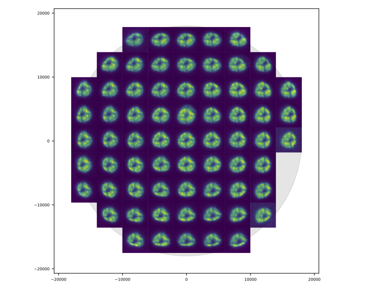
Figure 13 Donut data over an entire HSC field of view. The patterns have a smoothly varying structure across the field.

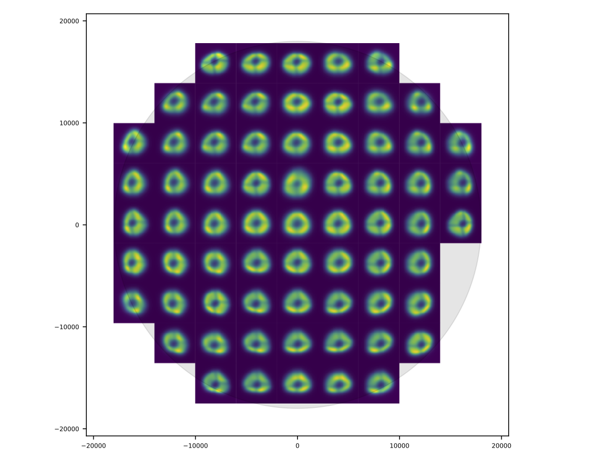
Figure 14 Best fitting models with \(j_\mathrm{max}=21\).

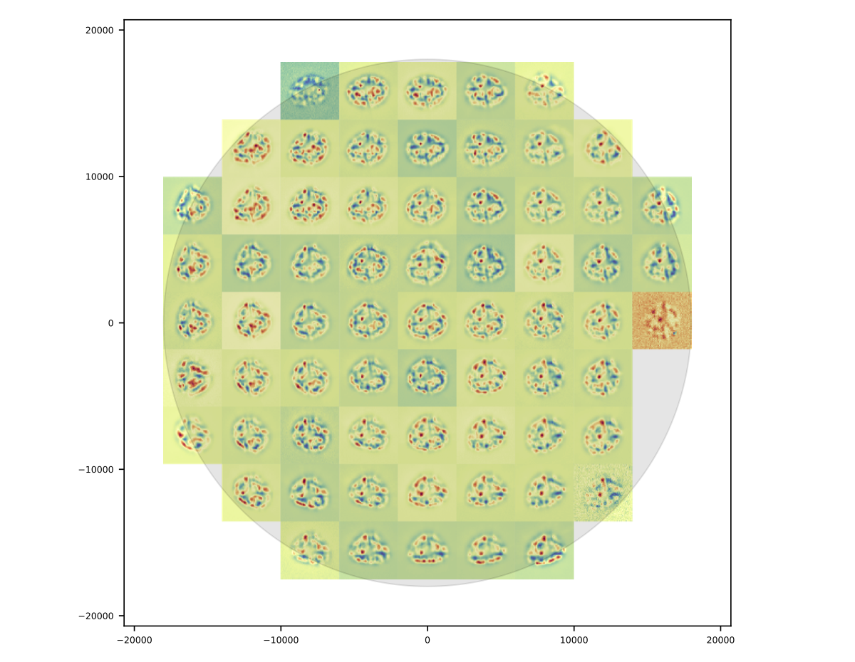
Figure 15 Residuals.

The residuals appear to vary smoothly over the focal plane. Features are coherent over scales of many CCDs (i.e., over 10s of arcminutes). Some features can even be picked out over most of the focal plane.

The longer the coherence scale of a feature, the closer to the pupil plane it must originate. That is, if features in the wavefront or wavefront residuals varied rapidly across the focal plane, they could not originate on the primary mirror or in the lower atmosphere, as these effect incoming beams roughly equally. Conversely, a given wavefront effect located near the focal plane or high up in the atmosphere will only affect a narrow range of focal plane positions (or equivalently, a narrow range of incoming angles).

Following this logic, it appears that a significant proportion of the wavefront residuals may originate near the Subaru primary mirror.

4.3.2   Wavefront¶

As in the Zemax tests, we predict the wavefront for in-focus images as the average of the inferred intra-focal and extra-focal wavefronts. (This assumes that the intra-focal and extra-focal camera displacements are precisely equal). The in-focus wavefront field-of-view variation, along with the pupil obscuration function are shown in the following figure.

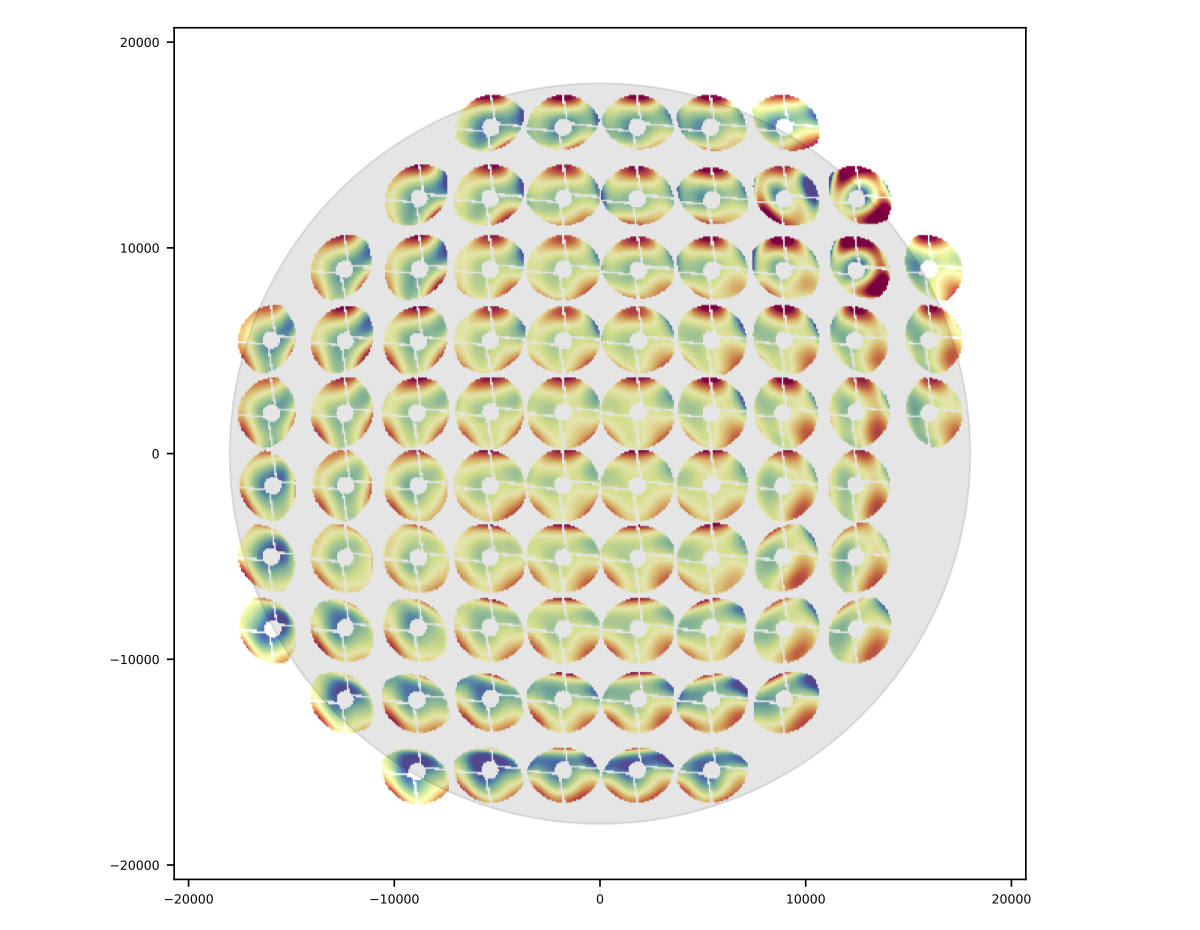
Figure 16 Model wavefront.

4.3.3   PSF¶

The purely optical PSF implied by the wavefront plotted above is shown below.

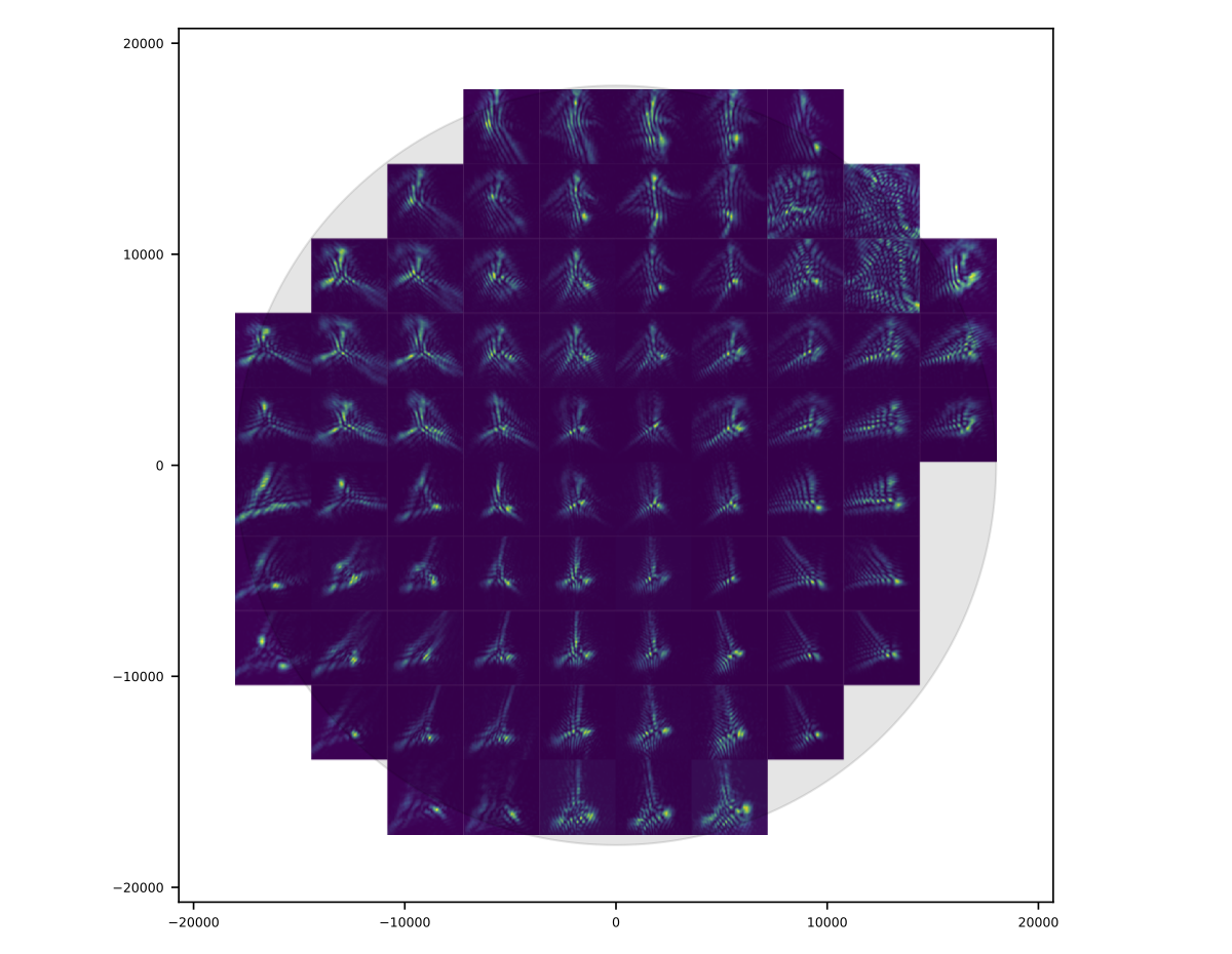
Figure 17 Model optical PSF. The size of each postage stamp is 0.64 arcseconds on a side.

4.3.4   Wavefront coefficients¶

Another way to look at these results is to plot the pupil plane wavefront coefficients as functions of focal plane location:

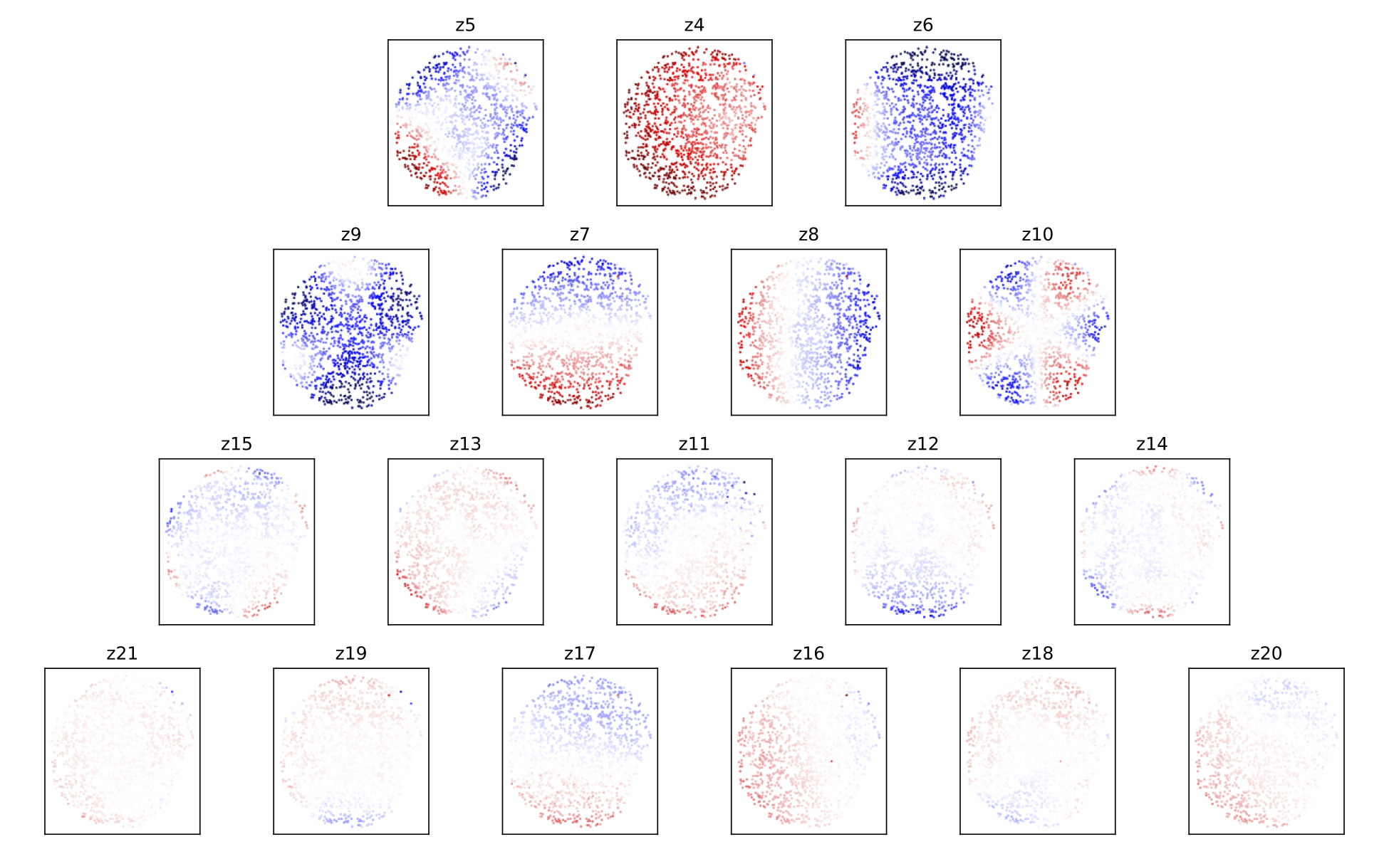
Figure 18 Wavefront coefficients across the focal plane.

The coefficients of Zernike polynomial terms that vary like \(\cos(n \theta_\mathrm{pupil})\) in the pupil show variation roughly proportional to \(\cos(n \theta_\mathrm{FOV})\) in the field of view. This is a simple consequence of the nearly circular symmetry of the HSC optical system. The amplitudes of the coefficients are also diminishing as the index increases, which hopefully means that despite the presence of significant residuals in the donut fits, we are capturing the most important wavefront features.

4.4   Model prediction comparison to measured PSFs¶

The triplets of extrafocal, intrafocal, and in-focus images enable a particular check on the accuracy of the wavefront-based optical PSF reconstruction. Since the in-focus images were taken nearly contemporaneously with the donut images on the same field, the state of the optics (other than focus) should be nearly identical in all three images of a triplet. The in-focus PSF contains a significant contribution from the atmosphere, of course, making a direct comparison of data to model difficult. However, if we approximate the atmospheric contribution as a convolution by a constant isotropic surface brightness profile, then we can convolve the model optics PSF by this fiducial atmospheric PSF to produce a profile more directly comparable to the in-focus data.

The plots below show predicted and observed moments of the PSF across the HSC field of view. The moments of each prediction and observation are summarized in “whiskers”, where the orientation of each whisker indicates the orientation of the PSF defined by:

\[\beta = \arctan(e_2, e_1)/2\]

and the length of each whisker indicates the ellipticity defined by:

\[e = \sqrt{e_1^2+e_2^2}\]

and \(e1\) and \(e2\) are related to the second moments of the PSF by

\[ \begin{align}\begin{aligned}e_1 = \frac{M_{xx} - M_{yy}}{M_{xx}+M_{yy}},\\e_2 = \frac{2 M_{xy}}{M_{xx}+M_{yy}}.\end{aligned}\end{align} \]

The whisker comparison plot for the triplet corresponding to the earlier figures in this section is immediately below, followed by whisker plots for the other available triplets.

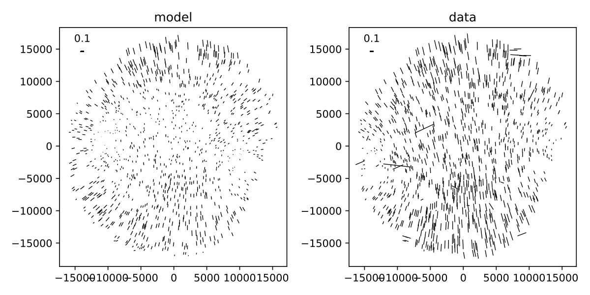
Figure 19 Whisker plot comparison for model derived from visits intra/extra focal visits 69028 and 69030 (left) and infocus data taken in visit 69026.

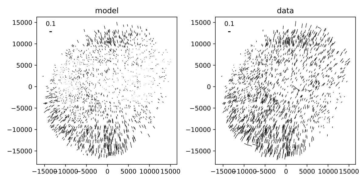
Figure 20 Whisker plot for triplet (69008/69010/69012).

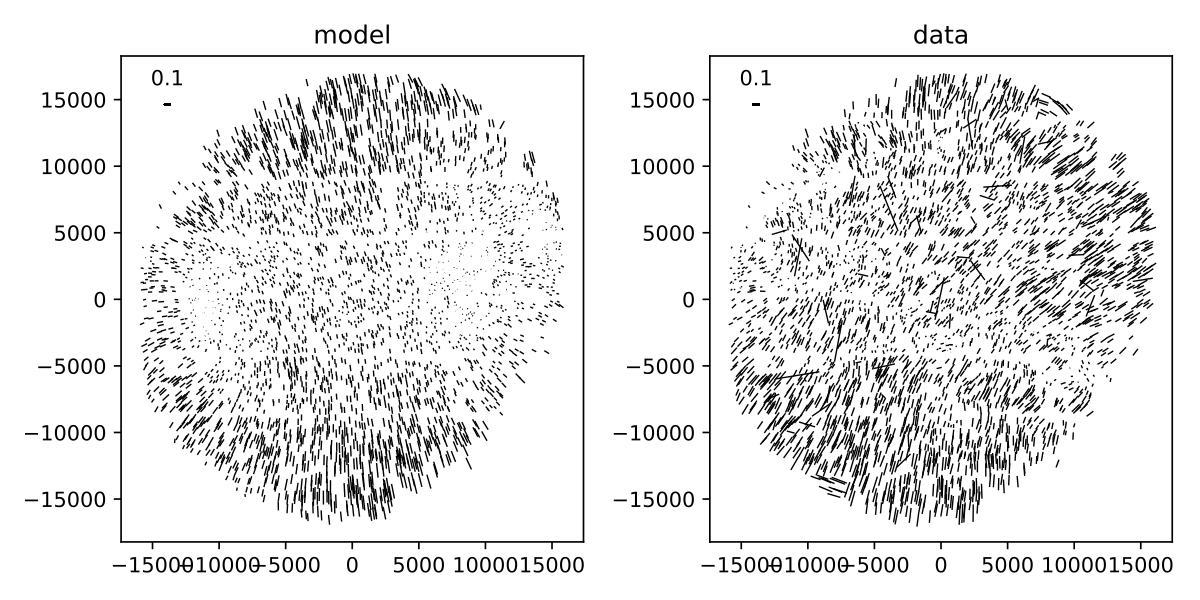
Figure 21 Whisker plot for triplet (69014/69016/69018).

Figure 22 Whisker plot for triplet (69032/69034/69036).

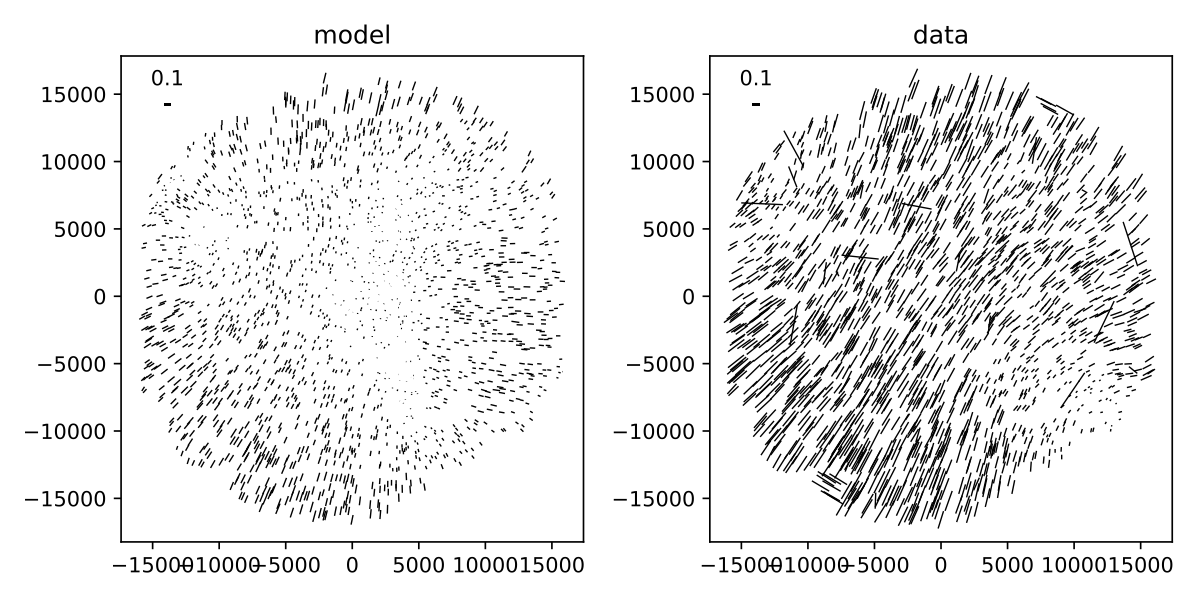
Figure 23 Whisker plot for triplet (69038/69040/69042).

Figure 24 Whisker plot for triplet (69050/69052/69054).

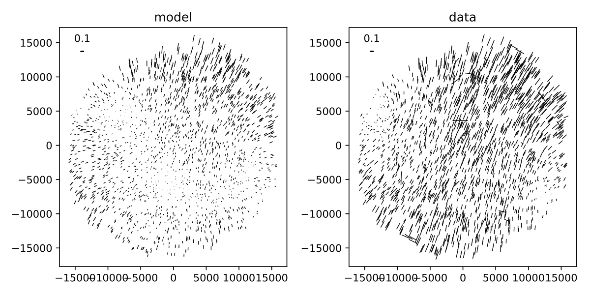
Figure 25 Whisker plot for triplet (69056/69058/69060).

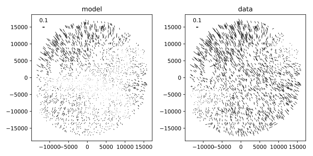
Figure 26 Whisker plot for triplet (69062/69064/69066).

The whisker plot comparisons show clear correlations between the predicted PSF moments and the observed PSF moments, indicating that we are on the right path towards optical PSF modeling. While the differences between predicted and observed whiskers are still under investigation, we would like to point out that the current model has no freedom for atmospheric variation across the field of view, or other contributions to the delivered PSF such as tracking errors / wind-shake, or effects originating in the sensors.

5   Open questions¶

A number of questions regarding donut-inferred wavefront analysis remain, which we list here:

• What is the impact of inferring the pupil obscuration function from the pinhole images?
• What is the impact of modeling donuts and PSFs monochromatically?
• How does distortion affect donuts or inferred in-focus PSFs?
• Would truncating the Zernike series at a larger order improve the fits? Would this improve the whisker plots?
• Can we verify in a ray-tracing package that misalignments really do only introduce changes in Zernike coefficients that vary slowly with field angle?